Blog Topics...

3D plotting (1) Academic Life (2) ACE (18) Adaptive Behavior (2) Agglomeration (1) Aggregation Problems (1) Asset Pricing (1) Asymmetric Information (2) Behavioral Economics (1) Breakfast (4) Business Cycles (8) Business Theory (4) China (1) Cities (2) Clustering (1) Collective Intelligence (1) Community Structure (1) Complex Systems (42) Computational Complexity (1) Consumption (1) Contracting (1) Credit constraints (1) Credit Cycles (6) Daydreaming (2) Decision Making (1) Deflation (1) Diffusion (2) Disequilibrium Dynamics (6) DSGE (3) Dynamic Programming (6) Dynamical Systems (9) Econometrics (2) Economic Growth (5) Economic Policy (5) Economic Theory (1) Education (4) Emacs (1) Ergodic Theory (6) Euro Zone (1) Evolutionary Biology (1) EVT (1) Externalities (1) Finance (29) Fitness (6) Game Theory (3) General Equilibrium (8) Geopolitics (1) GitHub (1) Graph of the Day (11) Greatest Hits (1) Healthcare Economics (1) Heterogenous Agent Models (2) Heteroskedasticity (1) HFT (1) Housing Market (2) Income Inequality (2) Inflation (2) Institutions (2) Interesting reading material (2) IPython (1) IS-LM (1) Jerusalem (7) Keynes (1) Kronecker Graphs (3) Krussel-Smith (1) Labor Economics (1) Leverage (2) Liquidity (11) Logistics (6) Lucas Critique (2) Machine Learning (2) Macroeconomics (45) Macroprudential Regulation (1) Mathematics (23) matplotlib (10) Mayavi (1) Micro-foundations (10) Microeconomic of Banking (1) Modeling (8) Monetary Policy (4) Mountaineering (9) MSD (1) My Daily Show (3) NASA (1) Networks (46) Non-parametric Estimation (5) NumPy (2) Old Jaffa (9) Online Gaming (1) Optimal Growth (1) Oxford (4) Pakistan (1) Pandas (8) Penn World Tables (1) Physics (2) Pigouvian taxes (1) Politics (6) Power Laws (10) Prediction Markets (1) Prices (3) Prisoner's Dilemma (2) Producer Theory (2) Python (29) Quant (4) Quote of the Day (21) Ramsey model (1) Rational Expectations (1) RBC Models (2) Research Agenda (36) Santa Fe (6) SciPy (1) Shakshuka (1) Shiller (1) Social Dynamics (1) St. Andrews (1) Statistics (1) Stocks (2) Sugarscape (2) Summer Plans (2) Systemic Risk (13) Teaching (16) Theory of the Firm (4) Trade (4) Travel (3) Unemployment (9) Value iteration (2) Visualizations (1) wbdata (2) Web 2.0 (1) Yale (1)

Saturday, December 22, 2012

Graph(s) of the Day

Suppose large number of identical firms in a perfectly competitive industry with constant returns to scale (CRTS) Cobb-Douglas production functions: \[Y = F(K, L) = K^{\alpha}(AL)^{1 - \alpha}\] Output, Y, is a homogenous of degree one function of capital, K, labor, L, and technology, A, is labor augmenting.

Typically, we economists model firms as choosing demands for capital and labor in order to maximize profits while taking prices as given (i.e., unaffected by the decisions of the individual firm):\[\max_{K,L} \Pi = K^{\alpha}(AL)^{1 - \alpha} - (wL + rK)\] where the prices are $1, w, r$. Note that I am following convention in assuming that the price of the output good is the numeraire (i.e., normalized to 1) and thus the real wage, $w$, and the return to capital, $r$, are both relative prices expressed in terms of units of the output good.

The first order conditions (FOCs) of a typical firms maximization problem are \[\begin{align}\frac{\partial \Pi}{\partial K}=&0 \implies r = \alpha K^{\alpha-1}(AL)^{1 - \alpha} \label{MPK}\\
\frac{\partial \Pi}{\partial L}=&0 \implies w = (1 - \alpha) K^{\alpha}(AL)^{-\alpha}A \label{MPL}\end{align}\] Dividing $\ref{MPK}$ by $\ref{MPL}$ (and a bit of algebra) yields the following equation for the optimal capital/labor ratio: \[\frac{K}{L} = \left(\frac{\alpha}{1 - \alpha}\right)\left(\frac{w}{r}\right)\] The fact that, for a given set of prices $w$, $r$, the optimal choices of $K$ and $L$ are indeterminate (any ratio of $K$ and $L$ satisfying the above condition will do) implies that the optimal scale of the firm is also indeterminate.

How can I create a graphic that clearly demonstrates this property of the CRTS production function? I can start by fixing values for the wage and return to capital and then creating contour plots of the production frontier and the cost surface.
The above contour plots are drawn for $w\approx0.84$ and $r\approx0.21$ (which implies an optimal capital/labor ratio of 2:1). You should recognize the contour plot for the production surface (left) from a previous post.  The contour plot of the cost surface (right) is a simple plane (which is why the isocost lines are lines and not curves!).  Combining the contour plots allows one to see the set of tangency points between isoquants and isocosts.

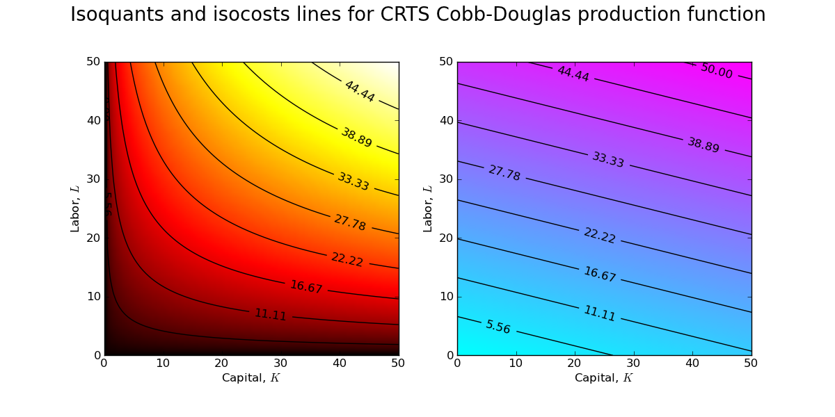
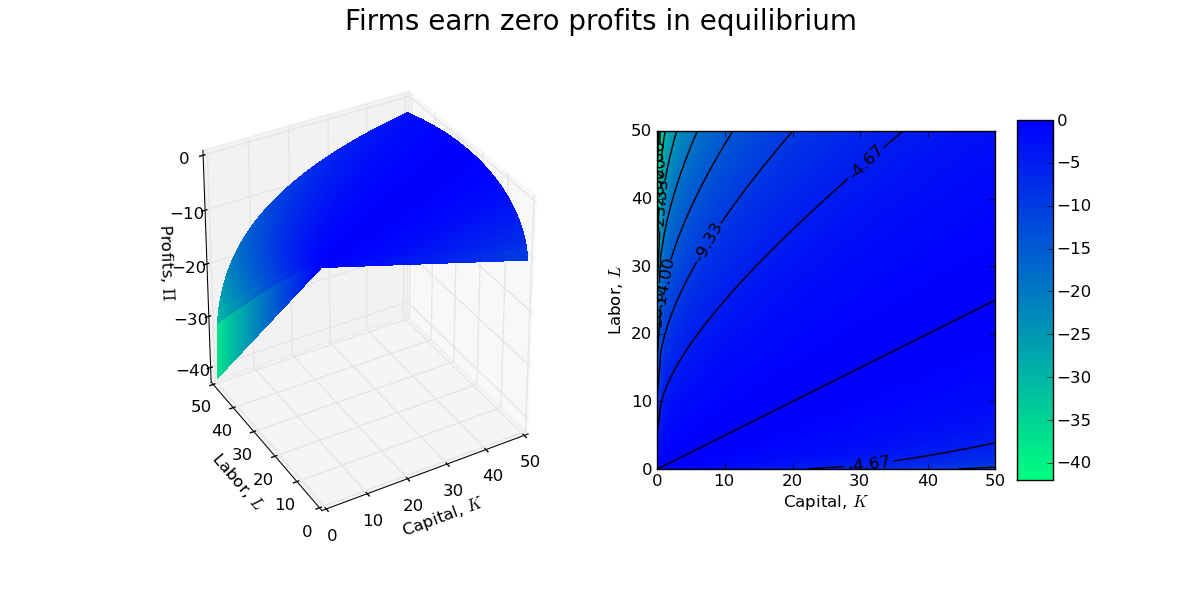
A firm manager is indifferent between each of these points of tangency, and thus the size/scale of the firm is indeterminate. Indeed, with CRTS a firm will earn zero profits at each of the tangency points in the above contour plot.


As usual, the code is available on GitHub.

Update: Installing MathJax on my blog to render mathematical equations was easy (just a quick cut and paste job).

No comments:

Post a Comment